Optimization and search are presented as pervasive ideas that span nature, everyday life, and large-scale engineered systems. From bees allocating foragers and building efficient combs to humans planning daily errands and companies routing fleets, the text motivates why optimization matters and when it is worth the effort. It frames optimization as systematic search over a feasible space defined by constraints, notes that benefits depend on problem scale and organizational readiness, and outlines a pragmatic path from small “toy” illustrations to real-world datasets and implementations. It also distinguishes decision timelines and performance needs across design (strategic), planning (tactical), and control (operational) problems, where time limits often force trade-offs between solution quality and speed.
The core ingredients of an optimization problem are clarified: decision variables (the choices), objective functions (what to maximize or minimize), and constraints (what must or should be satisfied). Solutions are categorized as feasible, optimal, or near-optimal, and search landscapes may contain global and local optima. The text highlights duality (maximization versus minimization) and notes that simple transformations of the objective do not move the optimizer. Through examples, it shows single-objective optimization (e.g., pricing for profit), multi-objective trade-offs (e.g., EV range versus acceleration, addressed via preferences or Pareto frontiers), and constraint-satisfaction problems that lack explicit objectives (e.g., n-queens). It also differentiates hard versus soft constraints and introduces penalty-based modeling, including adaptive penalties that tighten as search progresses.
Problem structure is used to separate well-structured problems (with clear states, operators, and tractable evaluation) from ill-structured problems (dynamic, partially observable, uncertain, and computationally intractable). A robotic pick-and-place task exemplifies a well-structured setting, whereas elevator dispatching illustrates an ill-structured one with an enormous state space and shifting goals; the traveling salesperson problem shows how something well-defined can still be intractable in practice. These realities motivate derivative-free, stochastic, black-box approaches that cope with nonlinearity, nonconvexity, and noise. Finally, the chapter emphasizes the central search dilemma—balancing exploration of new regions with exploitation of promising ones—explaining how overly exploitative local methods risk local traps, while purely random exploration is impractically slow, and effective algorithms manage the trade-off.
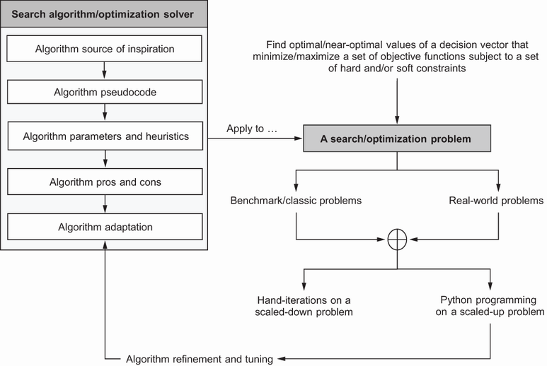
The book’s methodology—each algorithm will be introduced following a pattern that goes from explanation to application.
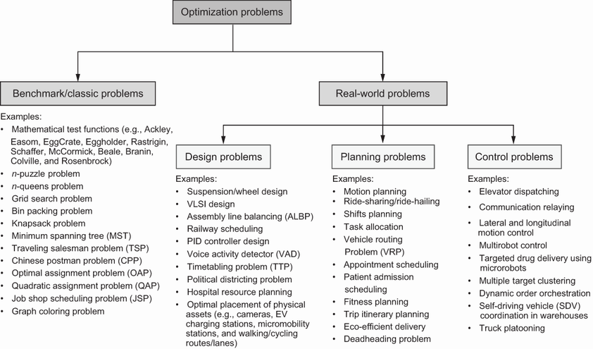
Examples of classic and real-world optimization problems
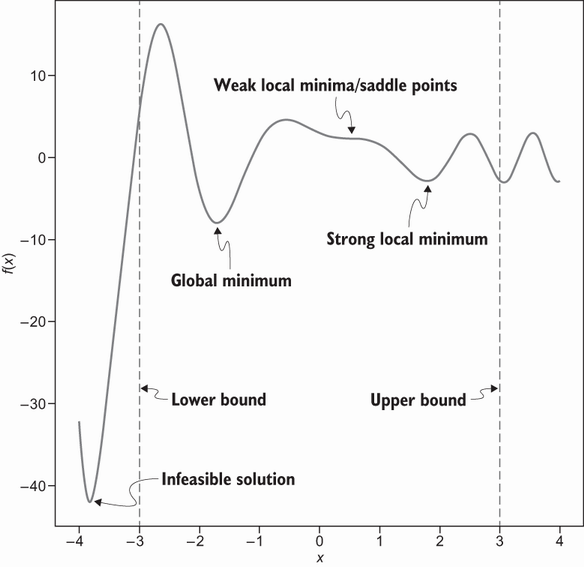
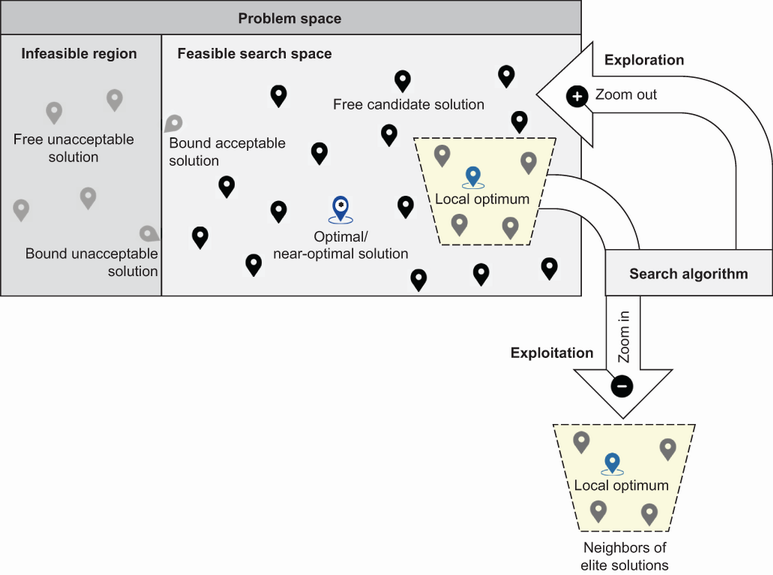
Feasible solutions fall within the constraints of the problem. A feasible search space may display a combination of global, strong local, and weak local minima.
Duality principle and mathematical operations on an optimization problem
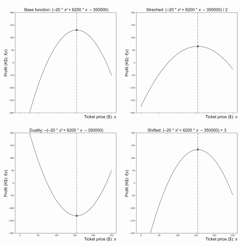
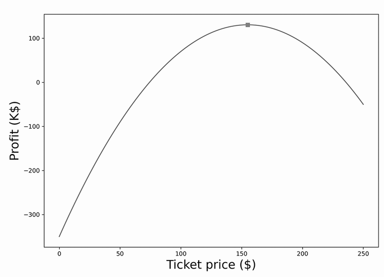
Ticket pricing problem—the optimal pricing that maximizes profit is $155 per ticket.
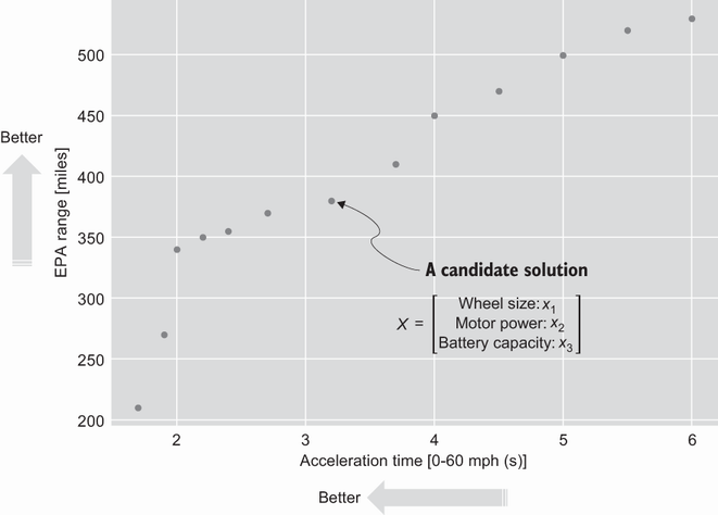
Electric vehicle design problem for maximizing EPA range and minimizing acceleration time
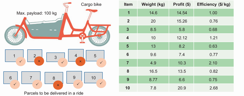
The cargo bike loading problem is an example of a problem with a soft constraint. While the weight of the packages can exceed the bike’s capacity, a penalty will be applied when the bike is overweight.
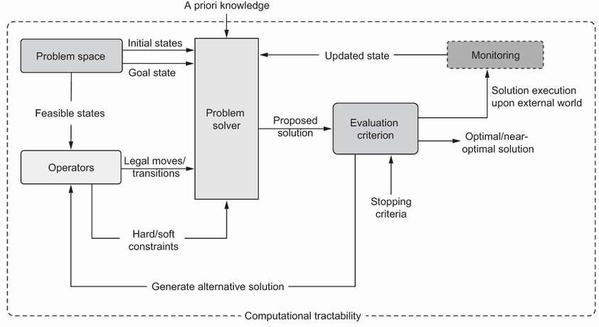
A WPS features a defined problem space, operators for allowable moves, clear evaluation criteria, and computational tractability.
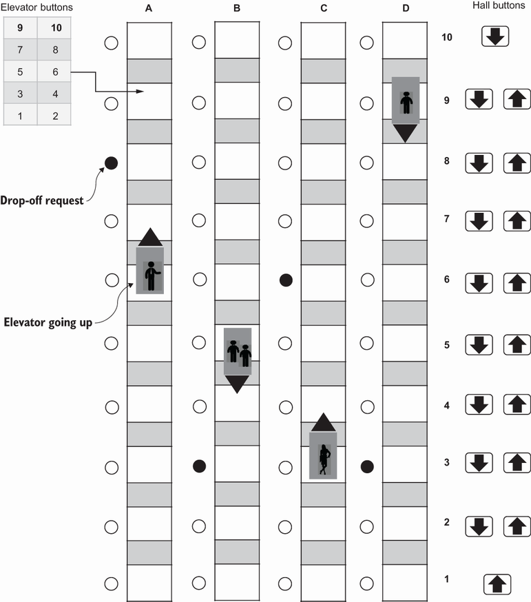
Elevator dispatching problem—with four elevator cars and 10 floors, this problem has ~1021 possible states.
Search dilemma—there is always a trade-off between branching out to new areas of the search space or focusing on an area with known good or elite solutions.
Summary
- Optimization is ubiquitous and pervasive in numerous areas of life, industry, and research.
- Decision variables, objective functions, and constraints are the main ingredients of optimization problems. Decision variables are the inputs that you have control over and that affect the objective function’s value. An objective function is the function that needs to be optimized, either minimized or maximized. Constraints are the limitations or restrictions that the solution must satisfy.
- Optimization is a search process for finding the “best” solutions to a problem, providing the best objective function values, and possibly subject to a given set of hard (must be satisfied) and soft (desirable to satisfy) constraints.
- Ill-structured problems are complex discrete or continuous problems without exact mathematical models and/or algorithmic solutions or general problem solvers. They usually have dynamic and/or partially observable large search spaces that cannot be handled by classic optimization methods.
- In many real-life applications, quickly finding a near-optimal solution is better than spending a large amount of time searching for an optimal solution.
- Two key concepts you’ll see frequently in future chapters are the exploration (or diversification) and exploitation (or intensification) search dilemmas. Achieving a trade-off between exploration and exploitation will allow the algorithm to find optimal or near-optimal solutions without getting trapped in local optima in an attractive region of the search space and without spending a large amount of time.
FAQ
What do we mean by "search" and "optimization" in this chapter?
Search is the systematic examination of states, starting from an initial state and aiming to reach a goal state. Optimization techniques are search methods whose goal is to find optimal or near-optimal states within the feasible search space (the subset of the problem space that satisfies all constraints).Why should I care about search and optimization?
- They are ubiquitous in nature (e.g., bee foraging, bird migration), daily life (planning a day, budgeting, workouts), and industry (logistics, telecom tower placement, ride-hailing dispatch, emergency response, airlines, healthcare, manufacturing, smart cities).
- Practicality matters: small problems (e.g., a pizzeria with ~10 nightly deliveries) may not justify complex optimization; for larger, high-impact problems (fleet assignment, crew scheduling), benefits can be substantial—but must be weighed against costs, expertise, and stakeholder follow-through.
How does the book go from toy problems to real-world solutions?
The book introduces each algorithm with intuition and pseudocode, identifies parameters and heuristics, and discusses pros/cons and adaptations. You first work small, hand-solved toy cases to see step-by-step mechanics, then scale up to real datasets with Python implementations and exercises to tune, evaluate performance, and study scalability.What are the basic ingredients of an optimization problem?
- Decision variables: the unknowns you choose (vector X) that define a candidate solution.
- Objective function(s): the quantity(ies) to optimize, often cast as minimization without loss of generality.
- Constraints: equalities/inequalities and variable bounds that define feasibility. Some constraints are hard (must hold), others are soft (desirable, often handled via penalties/rewards).
What types of solutions and optima should I expect in a search space?
- Feasible: satisfies all constraints.
- Optimal: feasible and provides the best objective value.
- Near-optimal: feasible and very good, but not necessarily the best.
- Optima types in minimization: global minimum (best over entire feasible space), strong local minimum (best in a neighborhood, but not global), weak local minimum (no better neighbors, but sequences can approach lower values).
Can you give a simple example of decision variables and objective functions?
Ticket pricing: demand Q = 5000 − 20x (x = ticket price). Revenue = Qx; Costs = a + Qb (a fixed, b variable per attendee). Profit f(x) = Revenue − Costs. With a = 50,000, b = 60, and price bounds 0 ≤ x ≤ 250, the profit is maximized at x = $155, yielding $130,500. Here, x is the decision variable; profit is the objective; price bounds are constraints.What is the difference between single-objective and multi-objective optimization, and how are multiple objectives handled?
- Single-objective: optimize one criterion (e.g., profit).
- Multi-objective: optimize several, often conflicting, criteria (e.g., minimize EV 0–60 time and maximize EPA range). Two common approaches:
- Preference-based scalarization: transform objectives (via duality if needed), then weight and combine them into one objective. Weight choice is subjective.
- Pareto optimization: find a set of nondominated trade-offs (Pareto frontier) and choose using higher-level preferences.
What are hard vs. soft constraints, and how do I model soft constraints?
- Hard constraints must be satisfied (e.g., no two classes in the same room at the same time; a teacher cannot teach two classes simultaneously; avoid ferries/tolls/highways if specified).
- Soft constraints are desirable but violable (e.g., minimum teaching days, nearby back-to-back rooms, avoiding rush-hour routes). They are typically modeled by adding rewards/penalties to the objective. Penalties can be dynamic—lighter early to encourage exploration, heavier later to enforce feasibility. Example: a cargo bike loading problem adds a fixed penalty if the total weight exceeds capacity.
How do well-structured problems differ from ill-structured problems?
- Well-structured problems (WSPs): have clear evaluation criteria, explicit problem spaces, defined operators, tractable computation, and readily available information. Example: a robotic pick-and-place cycle in a static, fully observable cell with a clear goal and timing criteria.
- Ill-structured problems (ISPs): have dynamic/partially observable spaces, unclear or shifting goals, limited models, contradictory solutions, uncertain data, and are often computationally intractable. Example: elevator dispatch with ~2.88 × 10^21 states and unpredictable calls; defining and maintaining an optimum is elusive.
- Some problems are WSPs in principle but ISPs in practice due to scale (e.g., TSP grows factorially—13 cities imply over 6.2 billion routes for naive enumeration; smarter methods reduce but do not eliminate complexity constraints).
 Optimization Algorithms ebook for free