This chapter offers a practical tour of core algorithmic ideas and data structures that underpin everyday software work and technical interviews. It emphasizes understanding trade-offs—how memory layout, access patterns, and operation costs shape real performance—and encourages benchmarking assumptions rather than relying solely on asymptotic analysis.
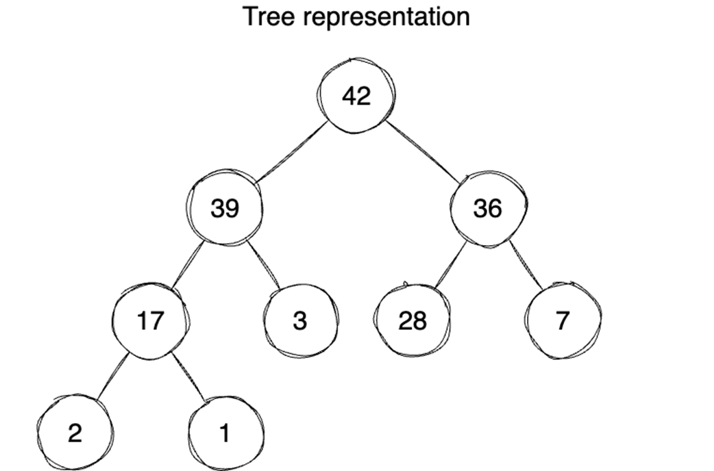
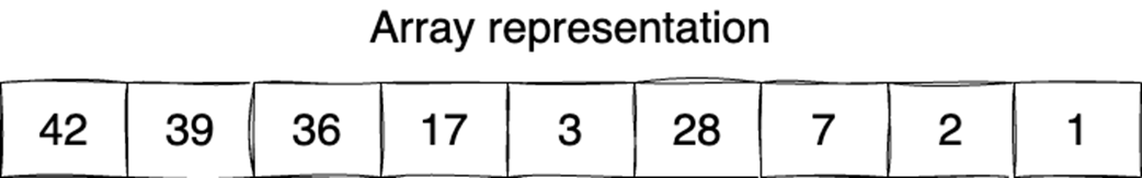
It begins by contrasting arrays and linked lists: arrays provide contiguous storage and O(1) indexed access but can be costly to resize (fixed arrays O(n), dynamic arrays amortized O(1) inserts with occasional O(n) resizes), while linked lists offer O(1) inserts/deletes at known positions at the expense of extra pointer memory and O(n) traversal. Despite theoretical wins, linked lists often underperform due to poor spatial locality, cache misses, and less predictable iteration (hindering prefetching and SIMD). The chapter then introduces binary heaps—complete trees maintaining a min- or max-heap property—typically implemented atop arrays with simple index arithmetic. Heaps support insert and extract in O(log n), find-min/max in O(1), and can be built in O(n). They excel for priority queues and often beat BSTs in practice thanks to cache-friendly layout and faster min/max access.
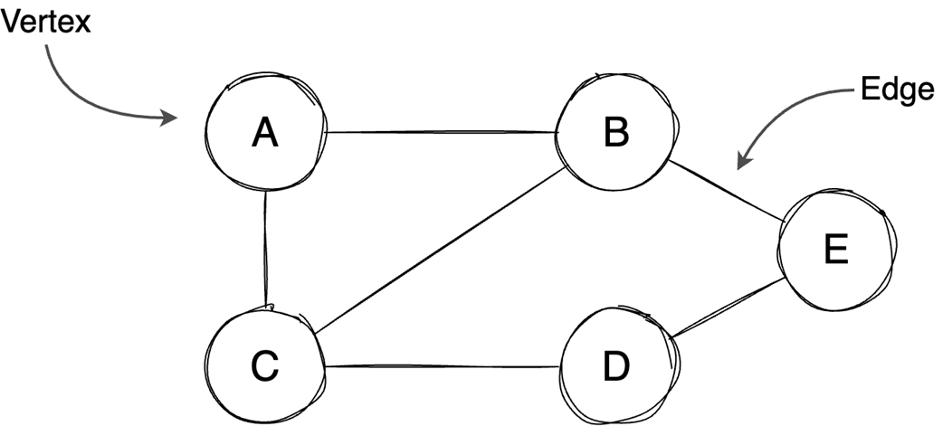
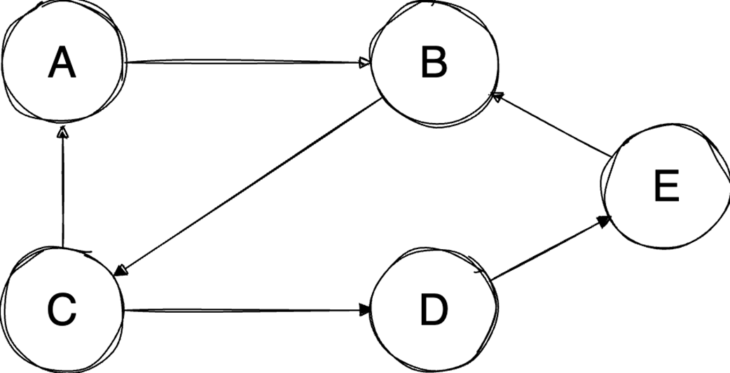
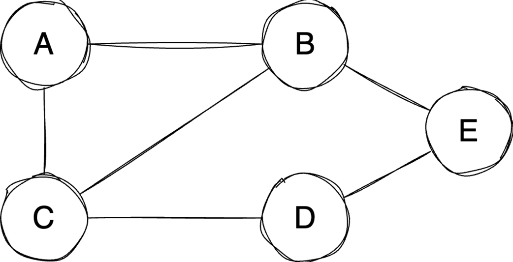
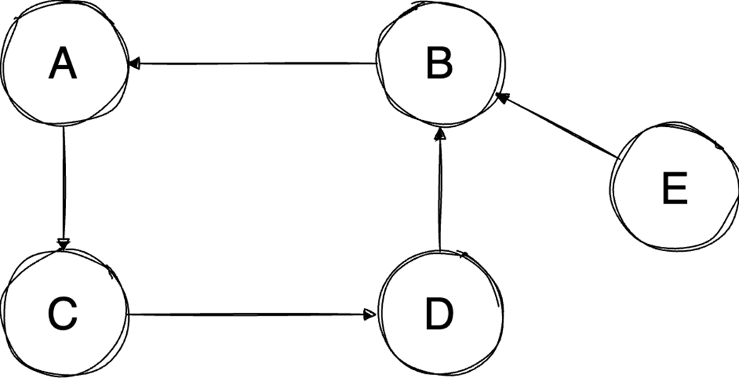
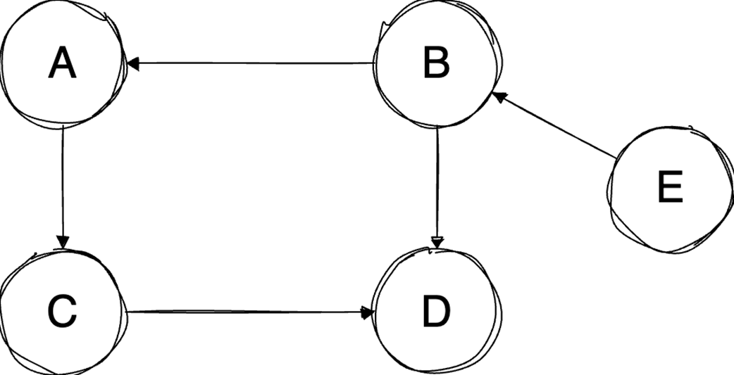
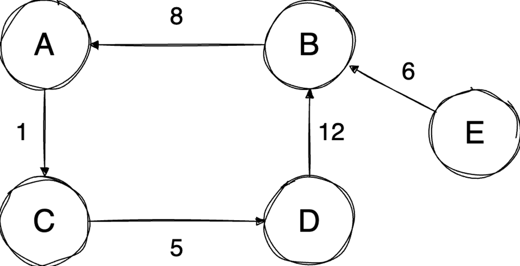
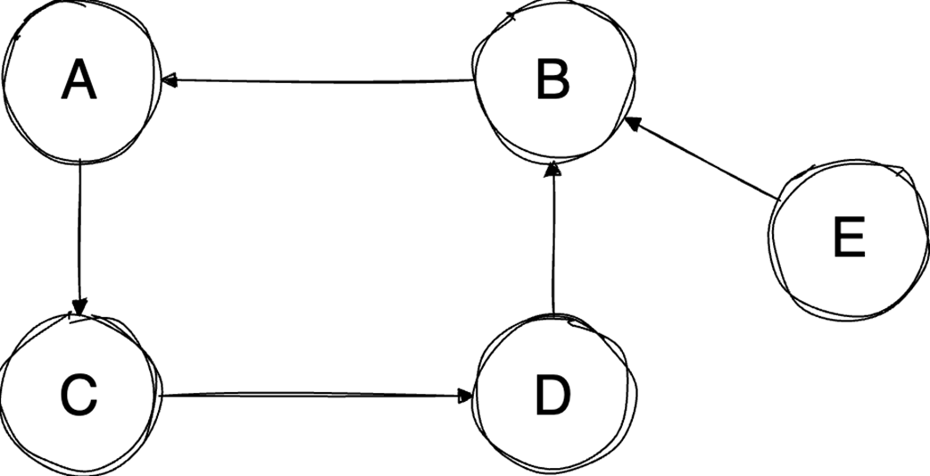
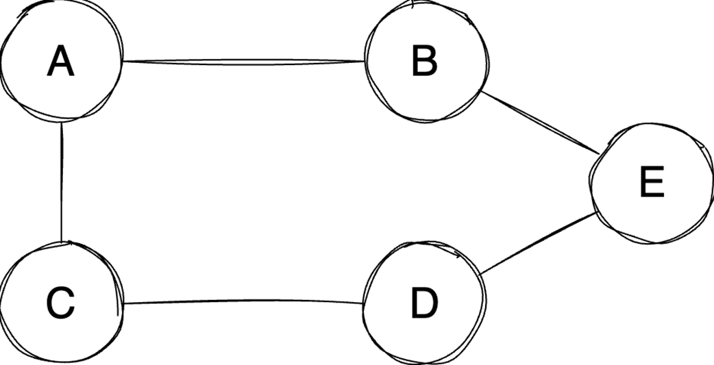
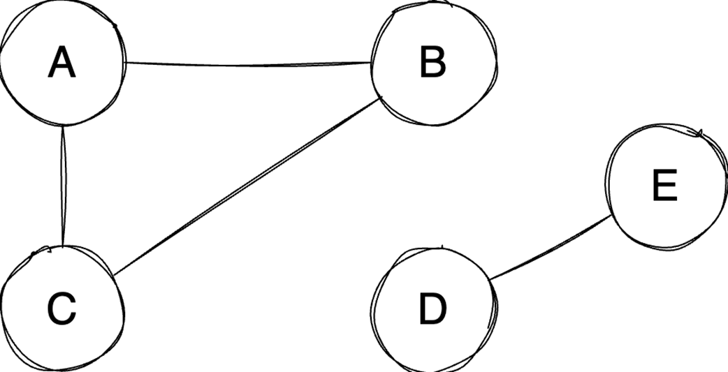
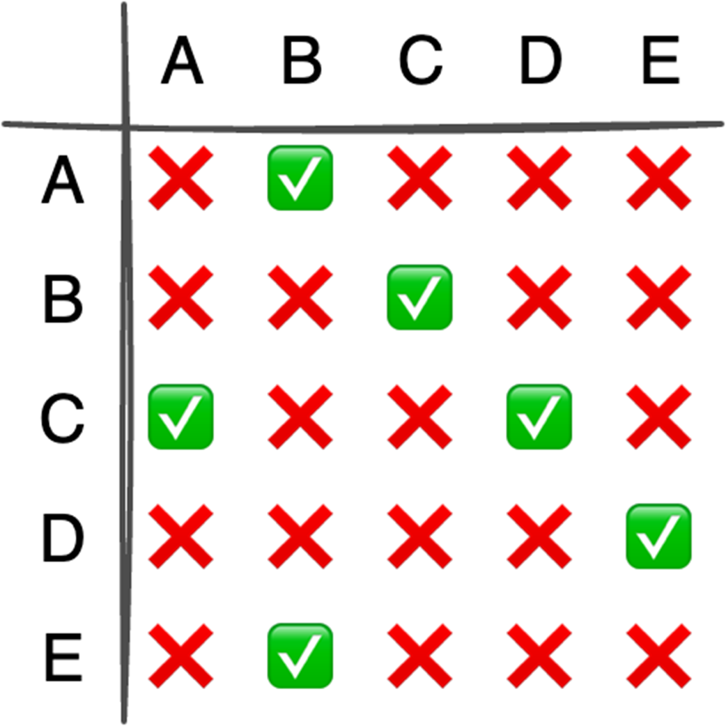
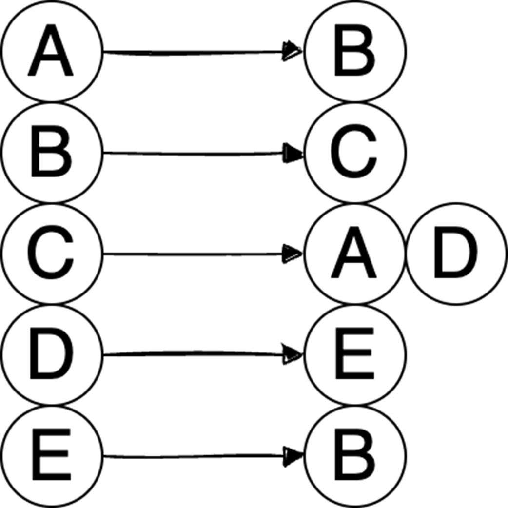
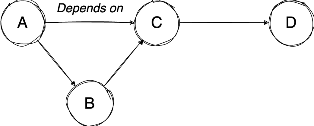
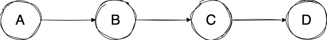
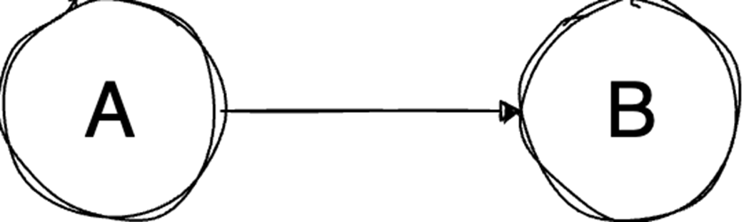
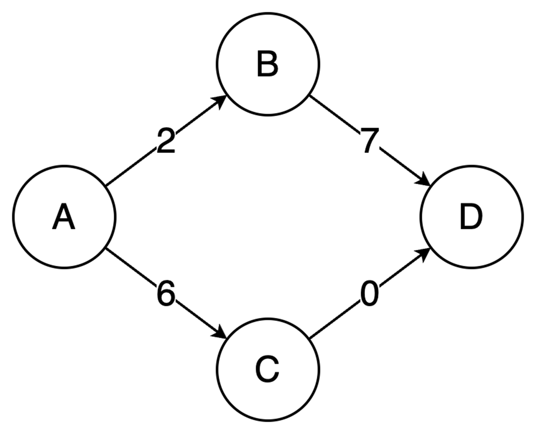
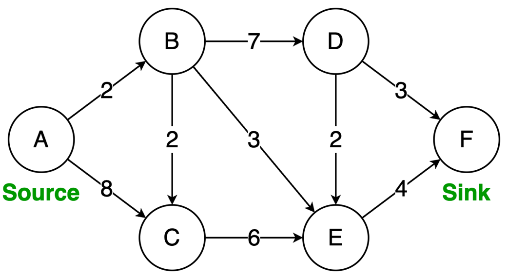
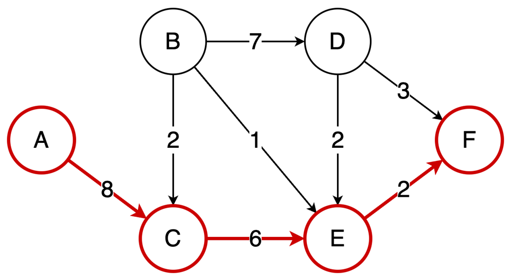
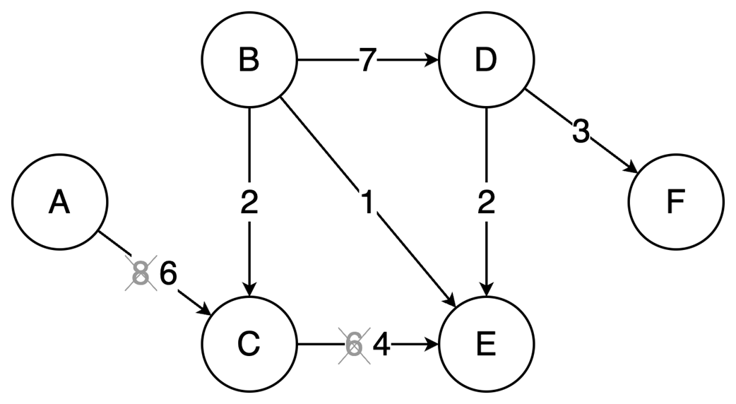
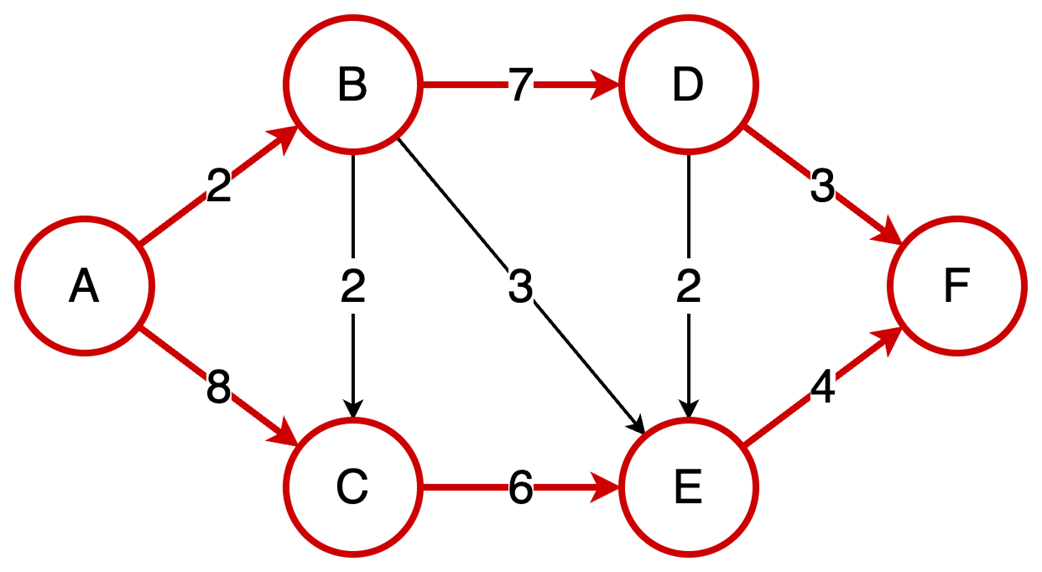
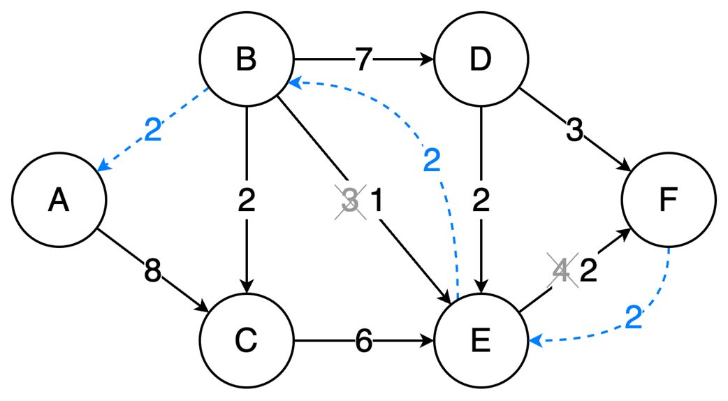
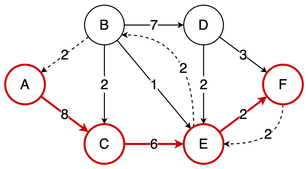
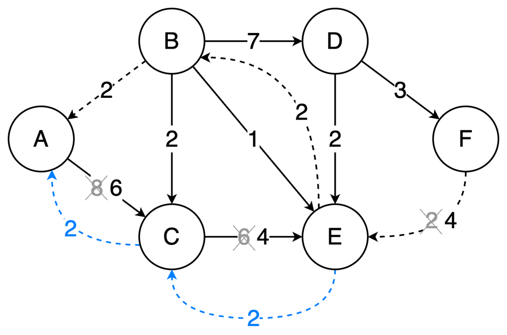
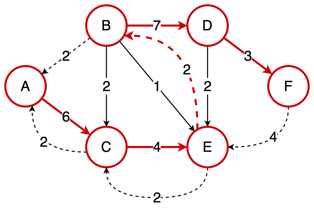
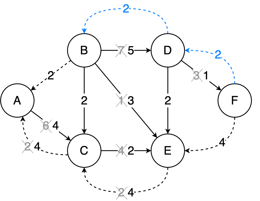
Next, it surveys graphs: what they model, key characteristics (directed/undirected, cyclic/acyclic, weighted/unweighted, connected/disconnected), and the trade-offs between adjacency matrices (O(1) edge queries, O(v²) space) and adjacency lists (O(v+e) space, edge lookups proportional to degree). It highlights essential algorithms—BFS for shortest paths in unweighted graphs, Floyd–Warshall for all-pairs shortest paths, and topological sort for DAGs via in-degrees and a zero-in-degree queue (O(v+e)) with applications in build systems, package managers, and deadlock detection. The chapter culminates with Ford–Fulkerson for max flow: repeatedly find augmenting paths, push the bottleneck flow, and update residual capacities—including crucial backward edges to enable flow redistribution—until no augmenting path remains. It notes the baseline time complexity O(E·U) and the Edmonds–Karp refinement using BFS to achieve O(V·E²), making the runtime depend only on graph size rather than the final flow value.
Summary
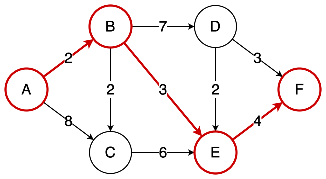
Ford-Fulkerson repeatedly finds augmenting paths and pushes flow through them.
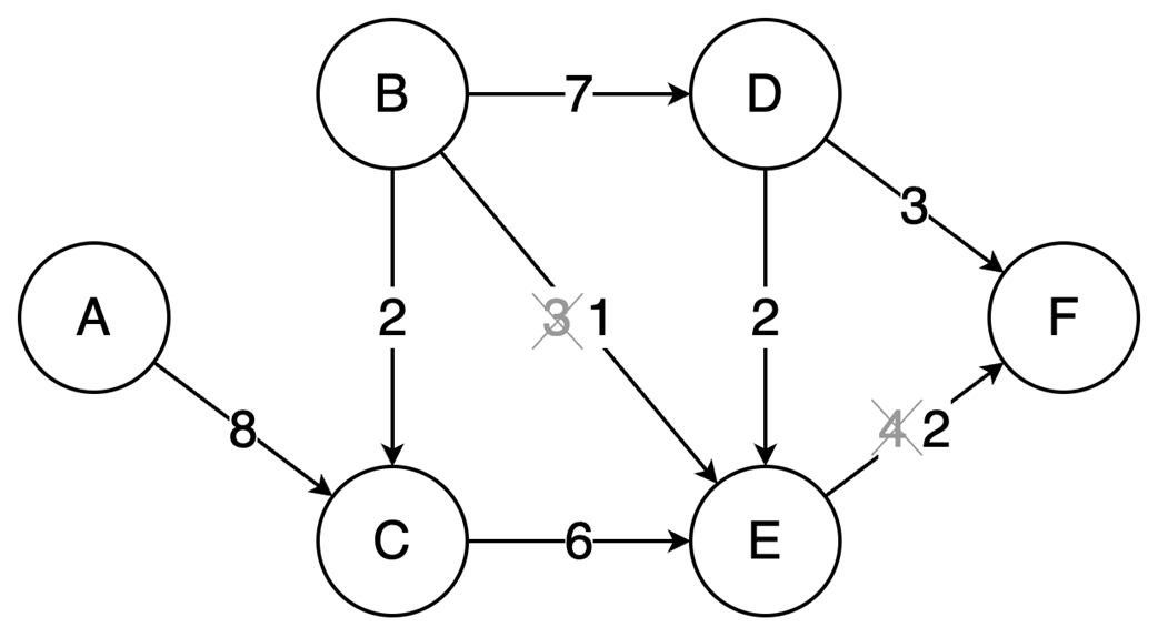
Backward edges allow redistribution of flow, which corrects any suboptimal choices made by selecting arbitrary augmenting paths.
The algorithm terminates when no more augmenting paths exist.
Using DFS, the time complexity is O(EU), which depends on the final solution, but switching to BFS (Edmonds-Karp variation) results in a time complexity of O(VE²), making it dependent only on the graph structure.
Arrays vs. linked lists: Pick for access vs. insertion/deletion patterns; mind cache locality.
Heaps provide O(1) peek min/max and O(log n) updates; great for priority queues.
Graphs model relationships; Choose representations (matrix/list) based on sparsity.
Topological sort orders DAGs by dependencies in O(V+E).
Ford‑Fulkerson finds max flow by augmenting paths and residual/backward edges.
FAQ
What are the key differences between arrays and linked lists, and when should I use each?Arrays store elements contiguously and support O(1) random access by index, making them fast to scan and cache-friendly. Linked lists store elements as nodes connected by pointers, which makes middle insertions/deletions O(1) when you already have a reference, but traversal is sequential. Use arrays (or dynamic arrays) for fast iteration and indexed access; prefer linked lists when you do frequent insertions/deletions away from the end.Why can linked lists be slower than arrays in real-world iteration?Linked lists often suffer from poor spatial locality: nodes are not guaranteed to be adjacent in memory, causing more cache misses and preventing effective CPU prefetching and SIMD vectorization. Even when allocated contiguously, pointer chasing and less predictable access patterns add overhead per iteration, making them slower than arrays in practice.What are the time complexities for common operations on arrays vs. linked lists?- Add: fixed array O(n); dynamic array amortized O(1) at the end but O(n) when resizing; linked list O(1) with a reference to the spot, otherwise O(n) to find it. - Delete: mirrors add. - Update: arrays O(1) by index; linked list O(1) with a node reference, otherwise O(n). - Find: O(n) for both when unsorted; arrays can do O(log n) binary search if sorted.What is a binary heap and when is it useful?A binary heap is a complete binary tree that satisfies the min-heap or max-heap property. It provides quick access to the smallest or largest element, making it ideal for priority queues and algorithms like Dijkstra’s and heapsort.How do array indices map to tree relationships in a binary heap?When a heap is stored in an array and a node is at index i: left child = 2*i + 1, right child = 2*i + 2, parent = (i - 1) / 2 (integer division).What are the time complexities of heap operations, and why is build-heap O(n)?insert: O(log n); getMin/getMax: O(1); extractMin/extractMax: O(log n); build-heap from an unsorted array: O(n) using bottom-up heapify-down, because most elements are near the leaves and require only a few swaps on average.When should I use a heap instead of a binary search tree (BST)?Choose a heap when you frequently need the global min or max: access is O(1) and updates are O(log n). Heaps build in O(n) and are array-based (cache-friendly). A balanced BST is better when you need ordered iteration and fast arbitrary searches (O(log n) lookups), not just min/max.What graph characteristics and in-memory representations should I know?Key characteristics: directed/undirected, cyclic/acyclic, weighted/unweighted, connected/disconnected. Representations: adjacency matrix gives O(1) edge tests but uses O(v²) space (great for dense graphs); adjacency list uses O(v + e) space with O(d) edge checks (best for sparse graphs).What is topological sort, when does it apply, and what is its complexity?Topological sort orders vertices of a Directed Acyclic Graph (DAG) so that all dependencies come before dependents. It typically uses in-degree counting with a queue of zero in-degree nodes and runs in O(v + e). It fails (detects) if a cycle exists.What is the Ford-Fulkerson algorithm, why are backward edges needed, and how does Edmonds–Karp differ?Ford-Fulkerson finds a maximum flow by repeatedly pushing flow along augmenting paths and updating residual capacities. It adds backward (residual) edges to allow flow redistribution if earlier choices were suboptimal. With arbitrary path selection (e.g., DFS), its time is O(E·U), where U is the max flow. Using BFS to pick shortest augmenting paths yields Edmonds–Karp with O(V·E²) time that depends only on graph size.
pro $24.99 per month
access to all Manning books, MEAPs, liveVideos, liveProjects, and audiobooks!
 The Coder Cafe ebook for free