1 Understanding foundation models

Foundation models mark a shift from building task- or dataset-specific models toward training a single, very large model on vast and diverse data that can be adapted to many tasks. Such models are characterized by four pillars: massive and varied training data, large parameter counts, broad task applicability, and the ability to be fine-tuned. In time series, this means one model can forecast across frequencies and temporal structures (trends, seasonality, holidays) and often support related tasks like anomaly detection or classification. The chapter also clarifies model versus algorithm, motivates why reuse reduces development overhead, and sets expectations that fine-tuning can tailor a general model to a particular domain while acknowledging that no single approach is best for every scenario.

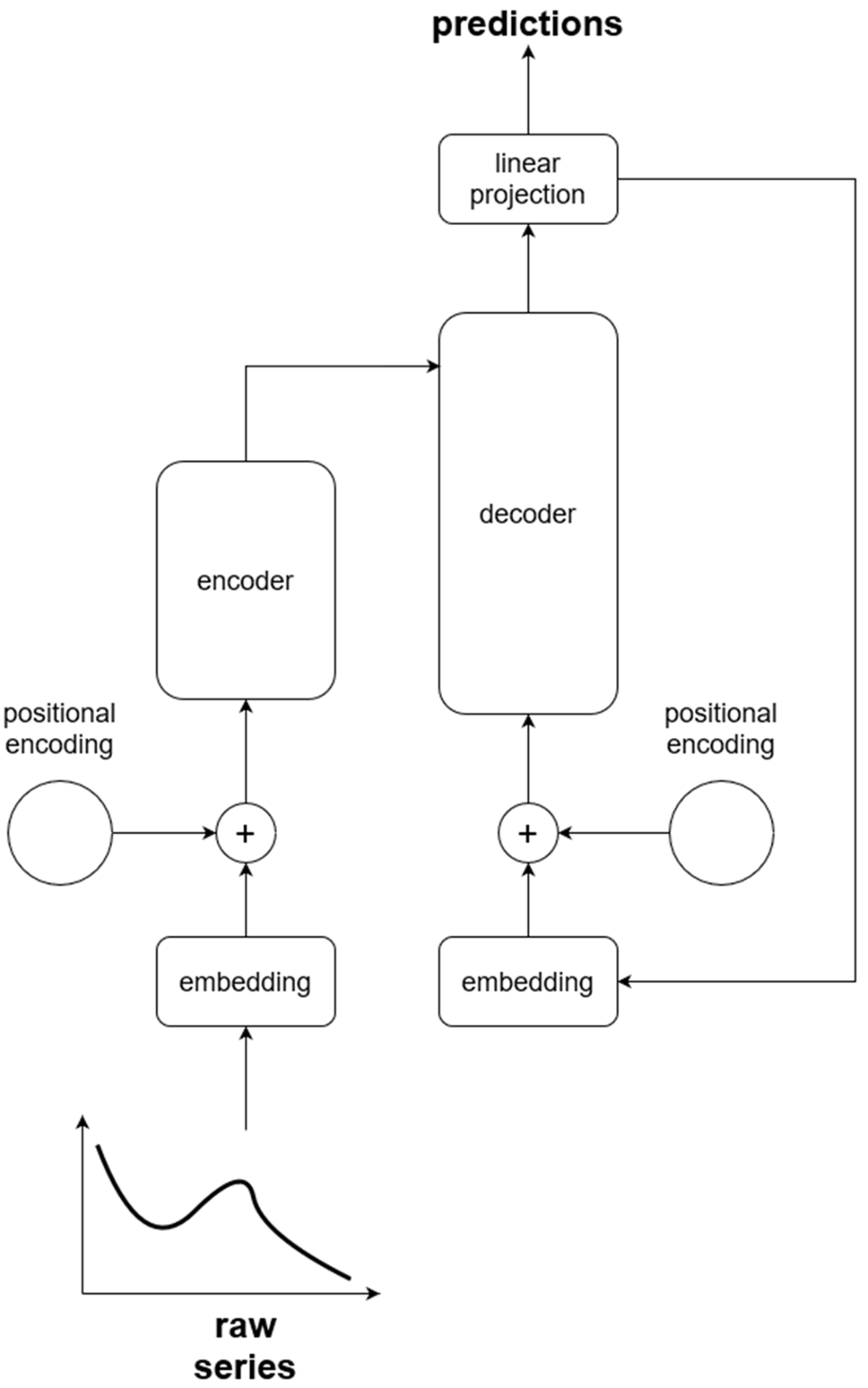
The chapter introduces the Transformer as the core architecture behind most foundation models and reframes it for time series forecasting. Inputs are tokenized and mapped through embeddings, then augmented with positional encoding to preserve temporal order. An encoder stack with multi-head self-attention learns rich dependencies across the sequence, while a decoder stack uses masked attention to prevent peeking into the future and cross-attention to leverage the encoder’s learned representation. Forecasts are produced autoregressively—each predicted step is fed back to inform subsequent steps—followed by a projection to output space. Understanding these components and their hyperparameters enables effective fine-tuning, capability assessment, and troubleshooting for different time series use cases.

Finally, the chapter weighs benefits and drawbacks of foundation forecasting models. Advantages include simple, out-of-the-box pipelines, usefulness with limited data, lower expertise requirements to get started, and broad reusability across tasks and datasets. Drawbacks include privacy and governance concerns (especially with hosted proprietary models), limited control over capabilities and horizons, potential mismatch to niche scenarios, and significant compute and storage demands. The book proceeds with hands-on exploration: building a small model to surface practical challenges; working with purpose-built time series models such as TimeGPT, Lag-LLaMA, Chronos, Moirai, and TimesFM; adapting language models (e.g., PromptCast, Time-LLM) for forecasting; and evaluating these approaches on real tasks like weekly sales forecasting and anomaly detection, culminating in a capstone comparison against statistical methods.

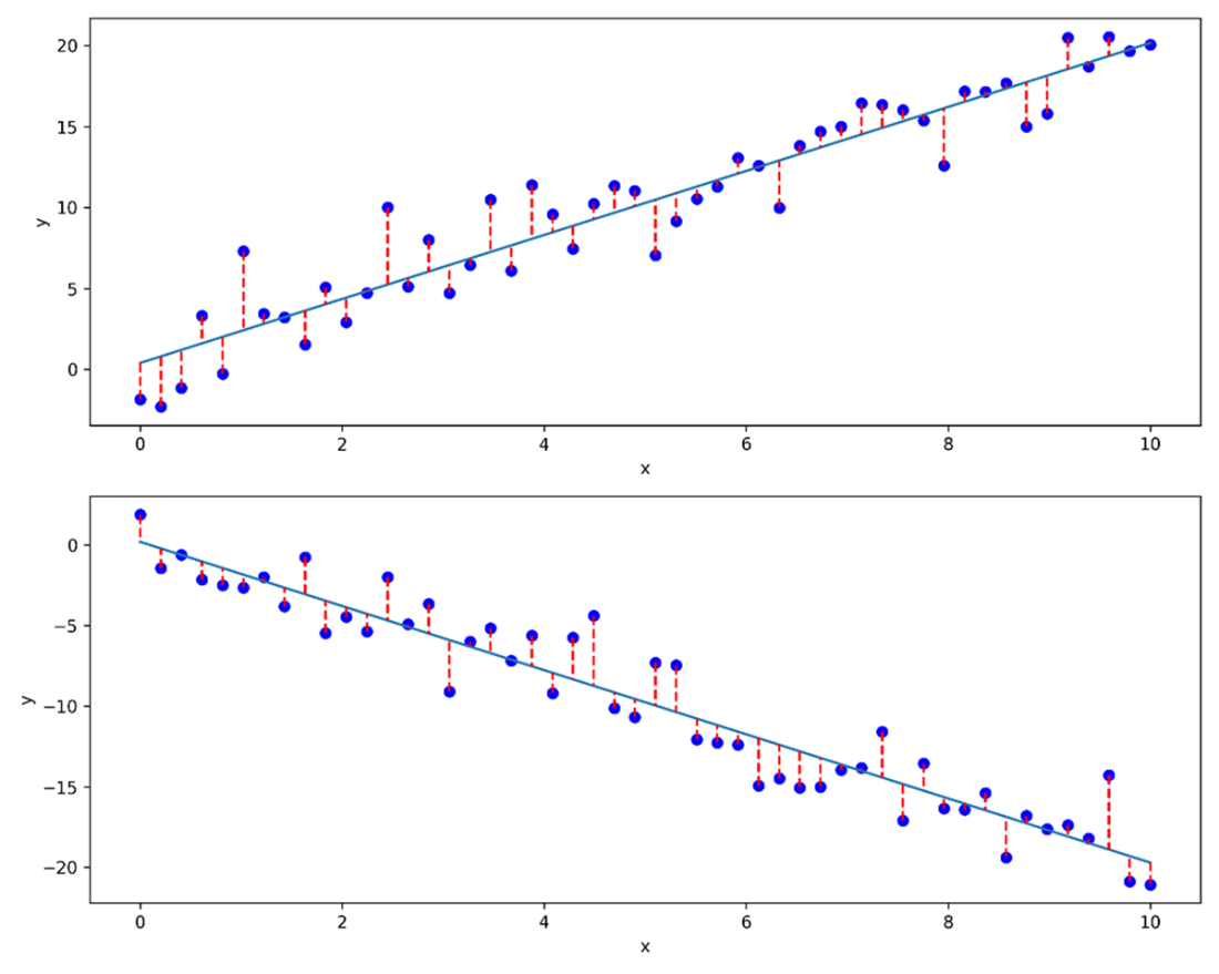
Result of performing linear regression on two different datasets. While the algorithm to build the linear model stays the same, the model is definitely very different depending on the dataset used.

Simplified Transformer architecture from a perspective of time series. The raw series enters at the bottom left of the figure, flows through an embedding layer and positional encoding before going into the decoder. Then, the output comes from the decoder one value at a time until the entire horizon is predicted.

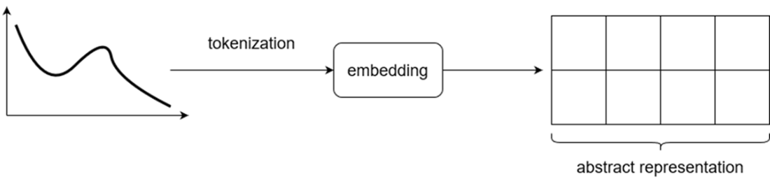
Visualizing the result of feeding a time series through an embedding layer. The input is first tokenized, and an embedding is learned. The result is the abstract representation of the input made by the model.

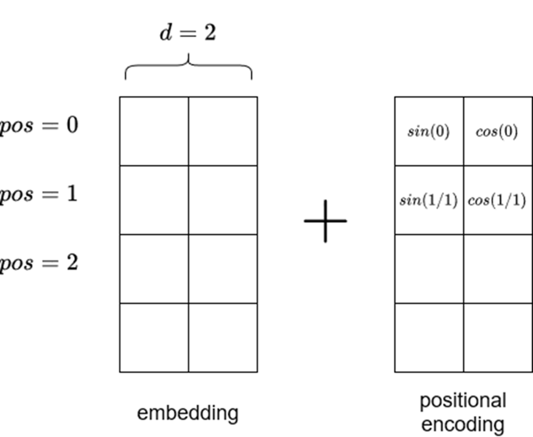
Visualizing positional encoding. Note that the positional encoding matrix must be of the same size as the embedding. Also note that sine is used in even positions, while cosine is used on odd positions. The length of the input sequence is vertical in this figure.

We can see that the encoder is actually made of many encoders which all share the same architecture. An encoder is made of a self-attention mechanism and a feed forward layer.

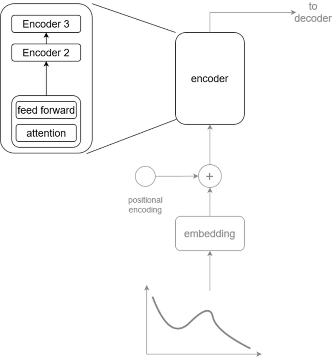
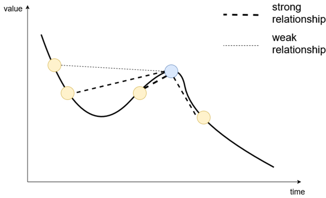
Visualizing the self-attention mechanism. This is where the model learns relationships between the current token (dark circle) and past tokens (light circles) in the same embedding. In this case, the model assigns more importance (depicted by thicker connecting lines) to closer data points than those farther away.

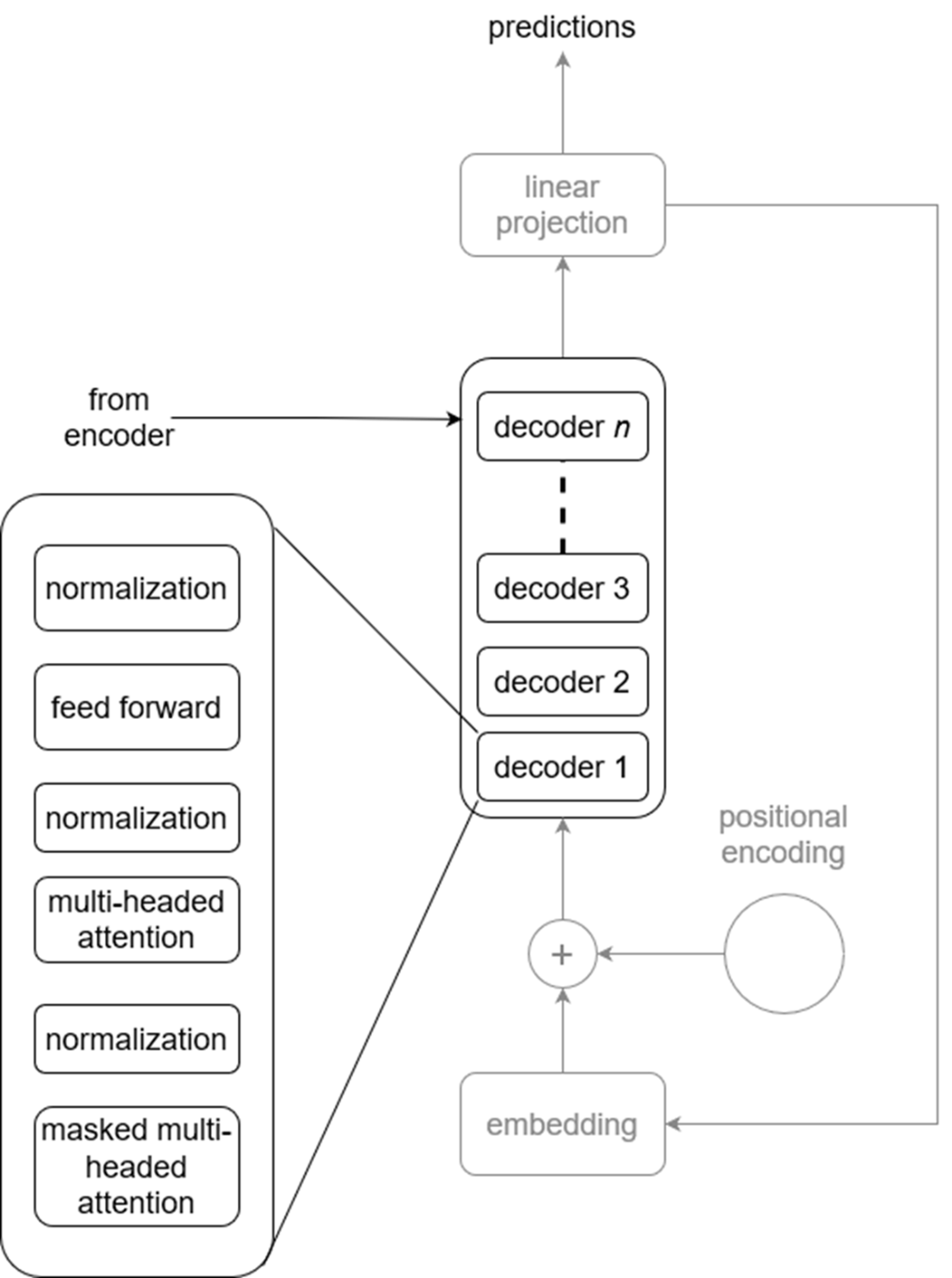
Visualizing the decoder. Like the encoder, the decoder is actually a stack of many decoders. Each is composed of a masked multi-headed attention layer, followed by a normalization layer, a multi-headed attention layer, another normalization layer, a feed forward layer, and a final normalization layer. The normalization layers are there to keep the model stable during training.

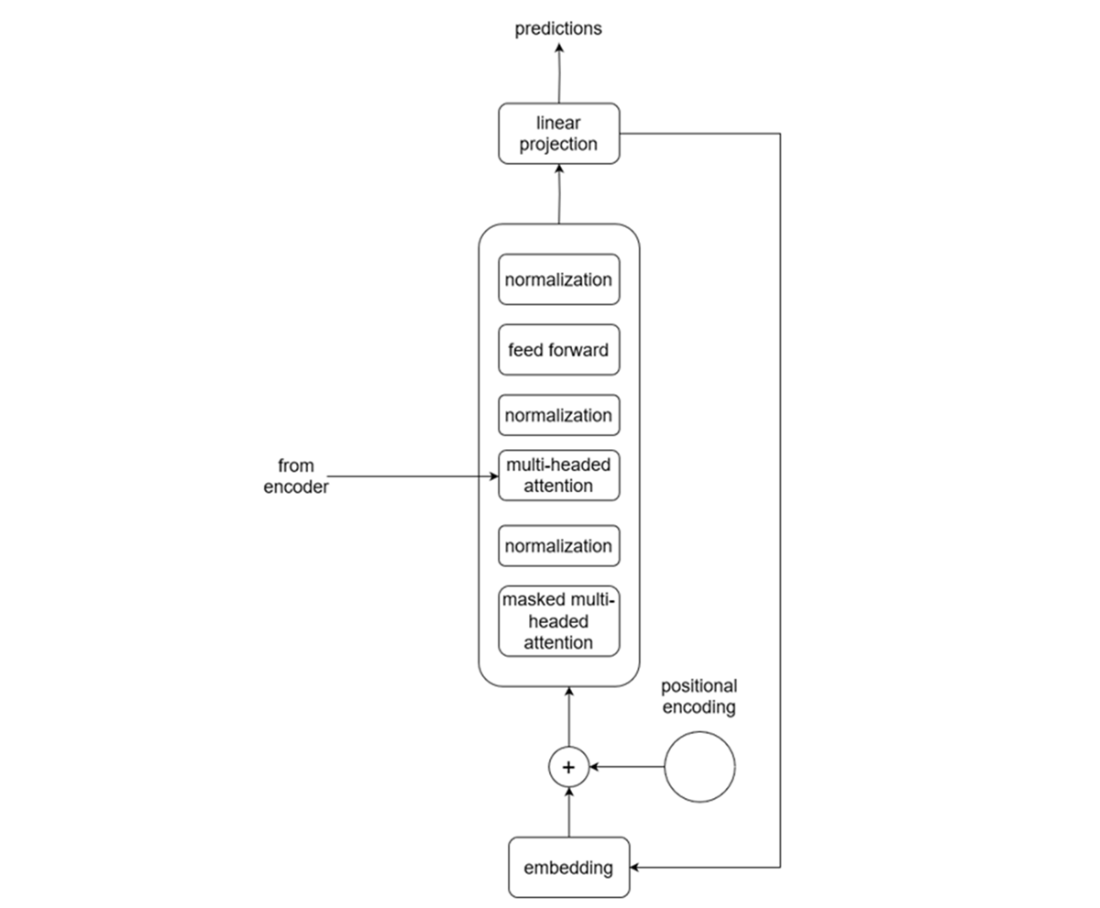
Visualizing the decoder in detail. We see that the output of the encoder is fed to the second attention layer inside the decoder. This is how the decoder can generate predictions using information learned by the encoder.

• A foundation model is a very large machine learning model trained on massive amounts of data that can be applied on a wide variety of tasks.
• Derivatives of the Transformer architecture are what powers most foundation models.
• Advantages of using foundation models include simpler forecasting pipelines, a lower entry barrier to forecasting, and the possibility to forecast even when few data points are available.
• Drawbacks of using foundation models include privacy concerns, and the fact that we do not control the model’s capabilities. Also, it might not be the best solution to our problem.
• Some forecasting foundation models were designed with time series in mind, while others repurpose available large language models for time series tasks.

FAQ